caledonia_co_nbm <- get_nbm_bl(geoid_co = "50005")
essex_co_nbm <- get_nbm_bl(geoid_co = "50009")
orleans_co_nbm <- get_nbm_bl(geoid_co = "50019")

nek_nbm <- bind_rows(
  caledonia_co_nbm,
  essex_co_nbm,
  orleans_co_nbm
)Here at the Center on Rural Innovation, we spend a lot of time thinking about broadband data. We’ve created detailed interactive maps of broadband service, produced research on the economic impacts of broadband on rural areas, and helped states and regions develop more equitable and effective broadband strategies. Now, we’re excited to share cori.data.fcc, an R package which makes Federal Communication Commission (FCC) broadband data releases more accessible than ever before.
In this blog post, I’ll cover three ways you can make use of our package to better understand broadband access and gaps.
1. View broadband service in your area
cori.data.fcc makes it easy to quickly pull data on broadband service for your area. In particular, using the get_nbm_bl function, you can access a CORI-opinionated version of the National Broadband Map’s latest release at the Census block level for any U.S. county.
In the example below, I pull NBM data for the “Northeast Kingdom” of Vermont, a region consisting of Caledonia, Essex, and Orleans counties, and then bind them together.
Here’s what the data looks like:
glimpse(nek_nbm)Rows: 4,363
Columns: 21
$ geoid_bl <chr> "500059570001000", "5000595700…
$ geoid_st <chr> "50", "50", "50", "50", "50", …
$ geoid_co <chr> "50005", "50005", "50005", "50…
$ cnt_total_locations <int> 1, 4, 5, 64, 3, 25, NA, 2, NA,…
$ cnt_bead_locations <int> 0, 4, 4, 51, 3, 23, NA, 2, NA,…
$ cnt_copper_locations <int> 0, 4, 2, 18, 3, 18, NA, 1, NA,…
$ cnt_cable_locations <int> 0, 0, 0, 0, 0, 0, NA, 0, NA, 0…
$ cnt_fiber_locations <int> 0, 0, 0, 0, 0, 0, NA, 0, NA, 0…
$ cnt_other_locations <int> 0, 0, 0, 0, 0, 0, NA, 0, NA, 0…
$ cnt_unlicensed_fixed_wireless_locations <int> 0, 0, 0, 0, 0, 0, NA, 0, NA, 0…
$ cnt_licensed_fixed_wireless_locations <int> 0, 2, 3, 46, 1, 14, NA, 2, NA,…
$ cnt_LBR_fixed_wireless_locations <int> 0, 0, 0, 1, 0, 2, NA, 0, NA, 0…
$ cnt_terrestrial_locations <int> 0, 4, 4, 51, 3, 23, NA, 2, NA,…
$ cnt_25_3 <int> 0, 1, 2, 40, 1, 5, NA, 0, NA, …
$ cnt_100_20 <int> 0, 0, 0, 0, 0, 0, NA, 0, NA, 0…
$ cnt_100_100 <int> 0, 0, 0, 0, 0, 0, NA, 0, NA, 0…
$ cnt_distcint_frn <int> NA, 3, 2, 4, 2, 4, NA, 2, NA, …
$ array_frn <list> <NULL>, <"0003645843", "00069…
$ combo_frn <dbl> NA, 3.040635e+18, 8.391679e+18…
$ release <date> 2024-06-01, 2024-06-01, 2024-…
$ state_abbr <chr> "VT", "VT", "VT", "VT", "VT", …If you are curious what those columns mean, you can use get_fcc_dictionary("nbm_block")
Next, we can pull spatial data using the tigris package to help us visualize the NBM data.
# Load all Vermont Census blocks
vt_blocks <- tigris::blocks("VT", progress_bar = FALSE)

# Load the Place boundary for the town of St. Johnsbury, VT
vt_places <- tigris::places(state = "VT", progress_bar = FALSE)
stj_vt <- vt_places %>% filter(GEOID == "5062125")
We’re going to take a look at broadband service in the town of St. Johnsbury, VT - one of the main towns in the region. To do so, we can filter to blocks that intersect with St. Johnsbury’s place boundary and then combine this data with NBM data to calculate the percent of locations in each block in St. Johnsbury that have 100/20 Mbps service, the FCC service benchmark for high speed broadband.
stj_vt_blocks <- vt_blocks %>%
  filter(lengths(st_intersects(., stj_vt)) > 0)

stj_vt_bb_blocks <- inner_join(
    stj_vt_blocks,
    nek_nbm,
    by = c("GEOID20" = "geoid_bl")
  ) %>%
  mutate(
    pct_100_20 = cnt_100_20 / cnt_total_locations
  )
Now that we’ve prepared our data, we can map it using ggplot to get a sense of the spatial trends of broadband access in St. Johnsbury.
bbox <- st_bbox(stj_vt_bb_blocks) %>%
      fit_bbox_to_aspect_ratio(target_aspect_ratio = 2)

fig <- ggplot(data = stj_vt_bb_blocks) +
  base_map(
    bbox,
    increase_zoom = 3,
    basemap = 'voyager'
  ) +
  geom_sf(aes(fill = pct_100_20), color = "dimgray", linewidth = .1, alpha = 0.9) +
  scale_fill_cori(
    discrete = FALSE,
    palette = "ctg2pu",
    labels = scales::label_percent(),
    reverse = T
  ) +
  coord_sf(
    expand = TRUE,
    xlim = c(bbox['xmin'], bbox['xmax']),
    ylim = c(bbox['ymin'], bbox['ymax'])
  ) +
  theme_cori_map() +
  theme(
    legend.key.width = unit(50, "pt"),
  ) +
  labs(
    title = "Broadband service in St. Johnsbury, VT",
    subtitle = "Percent of locations with access to 100/20 Mbps service by census block",
    caption = "Data source: 2023 FCC National Broadband Map\nMap source: © OpenStreetMap contributors © CARTO"
  )

save_plot(fig, here("images/st_j_bb_service.png"), chart_height = 8)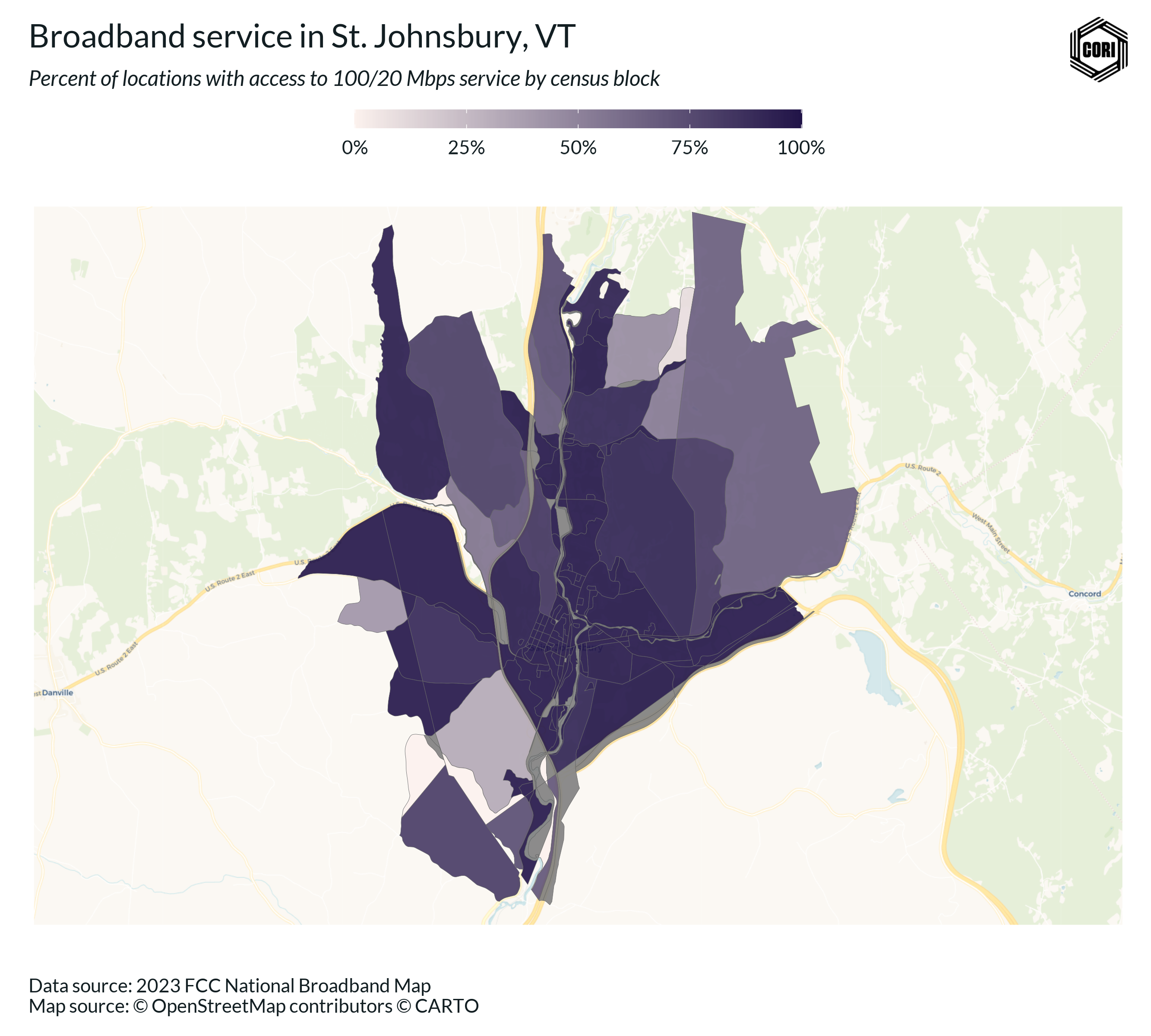
We can also easily plot broadband service data for the entire Northeast Kingdom.
# Get Census block BB data for the Northeast Kingdom
nek_bb_blocks <- inner_join(
    vt_blocks,
    nek_nbm,
    by = c("GEOID20" = "geoid_bl")
  ) %>%
  mutate(
    pct_100_20 = cnt_100_20 / cnt_total_locations,
    pct_fiber = cnt_fiber_locations / cnt_total_locations
  )

# Get major NEK Place centroids for map labeling
vt_places_centroids <- vt_places %>%
  st_as_sf() %>%
  st_centroid() %>%
   filter(lengths(st_intersects(., nek_bb_blocks)) > 0)
bbox <- st_bbox(nek_bb_blocks) %>%
fit_bbox_to_aspect_ratio(target_aspect_ratio = 2)
fig <- ggplot(data = nek_bb_blocks) +
base_map(
bbox,
increase_zoom = 3,
basemap = 'voyager'
) +
geom_sf(aes(fill = pct_100_20), color = "dimgray", linewidth = 0.1, alpha = 0.9) +
scale_fill_cori(
discrete = FALSE,
palette = "ctg2pu",
labels = scales::label_percent(),
reverse = T
) +
geom_sf_label(data = vt_places_centroids,
aes(label = NAME), size = 2, color = "black", family = "Lato", fontface = "bold") +
coord_sf(
expand = TRUE,
xlim = c(bbox['xmin'], bbox['xmax']),
ylim = c(bbox['ymin'], bbox['ymax'])
) +
theme_cori_map() +
theme(
legend.key.width = unit(50, "pt"),
) +
labs(
title = "Broadband service in the Northeast Kingdom",
subtitle = "Percent of locations with access to 100/20 Mbps service by census block",
caption = "Data source: 2023 FCC National Broadband Map\nMap source: © OpenStreetMap contributors © CARTO",
x = NULL,
y = NULL
)
save_plot(fig, here("images/nek_bb_service.png"), chart_height = 8)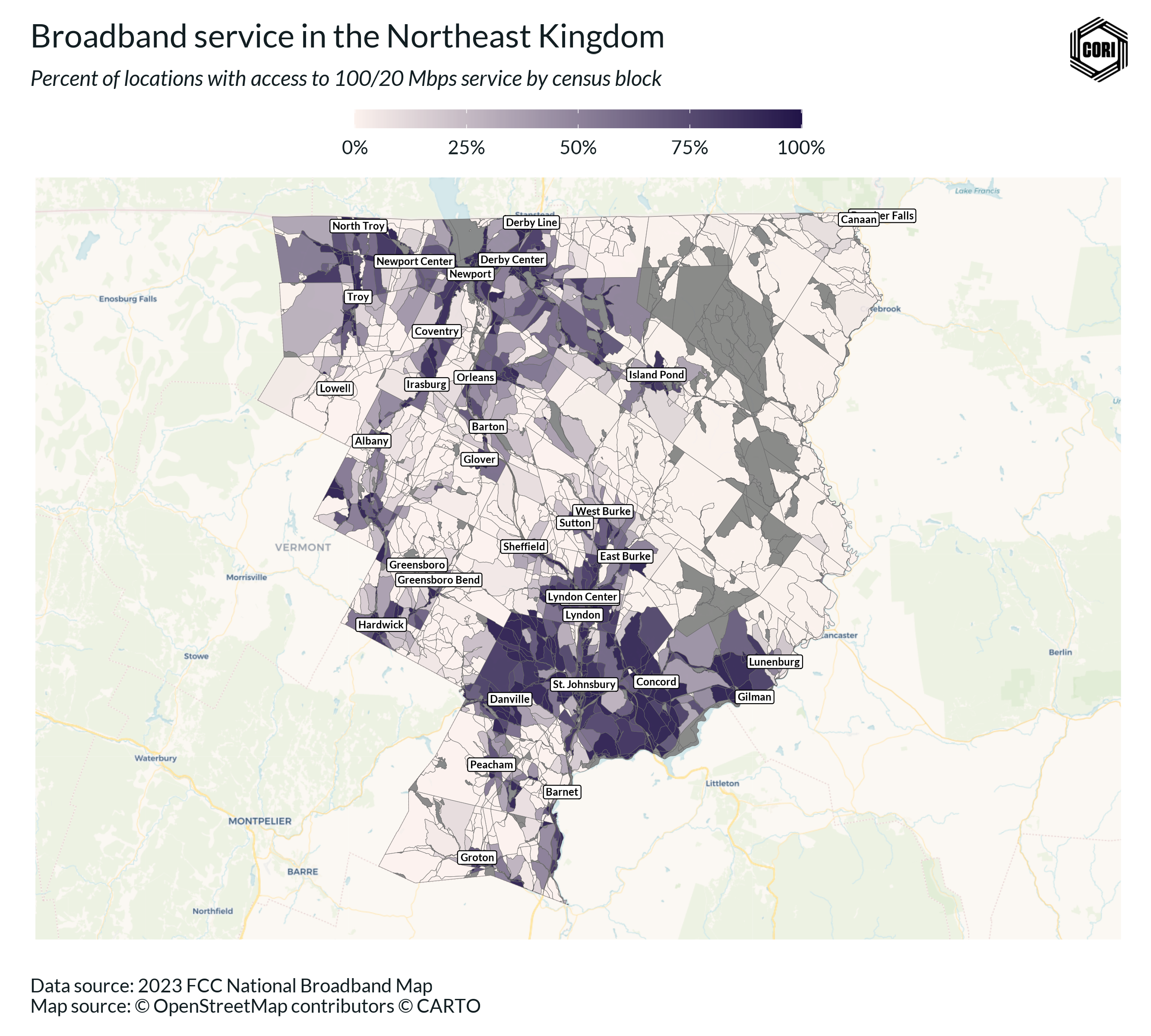
Broadband access can also be analyzed by technology, including fiber, cable, and fixed wireless. This example map focuses on fiber access in the region.
fig <- ggplot(data = nek_bb_blocks) +
  base_map(
    bbox,
    increase_zoom = 3,
    basemap = 'voyager'
  ) +
  geom_sf(aes(fill = pct_fiber), color = "dimgray", linewidth = 0.1, alpha = 0.6) +
  scale_fill_cori(
    discrete = FALSE,
    palette = "ctg2pu",
    labels = scales::label_percent(),
    reverse = T
  ) +
  geom_sf_label(data = vt_places_centroids,
                aes(label = NAME), size = 2, color = "black", family = "Lato", fontface = "bold") +
  coord_sf(
    expand = TRUE,
    xlim = c(bbox['xmin'], bbox['xmax']),
    ylim = c(bbox['ymin'], bbox['ymax'])
  ) +
  theme_cori_map() +
  theme(
    legend.key.width = unit(50, "pt"),
  ) +
  labs(
    title = "Fiber access in the Northeast Kingdom",
    subtitle = "Percent of locations with access to fiber by census block",
    caption = "Data source: 2023 FCC National Broadband Map\nMap source: © OpenStreetMap contributors © CARTO",
    x = NULL,
    y = NULL
  )

save_plot(fig, here("images/nek_fiber_service.png"), chart_height = 8)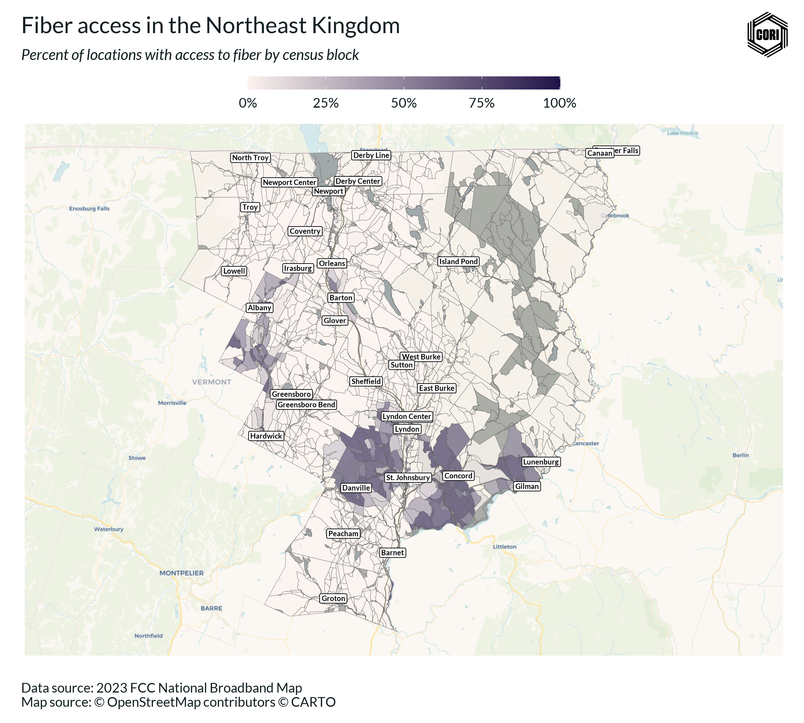
Fiber service is pretty rare! Only a handful of towns have access.
Next, let’s generate some summary statistics to see what percent of locations in the region have fiber access.
# Calculate share of locations with access to fiber
nek_locations_total <- nek_bb_blocks %>%
  pull(cnt_total_locations) %>%
  sum(na.rm = T)

nek_locations_fiber <- nek_bb_blocks %>%
  pull(cnt_fiber_locations) %>%
  sum(na.rm = T)

nek_locations_fiber / nek_locations_total
Turns out only 11.5% locations have fiber access in the Northeast Kingdom.
2. View Internet Service Provider (ISP) footprints
cori.data.fcc can also be used to better understand ISP presence in an area. Let’s explore how by first pulling Form 477 data for the state of Vermont.
# Pulling all Form 477 for the state of Vermont
vt_477 <- get_f477("VT", frn = "all")
In this example, I’m interested in seeing the footprint for NEK Broadband, a community non-profit bringing high-speed broadband to the Northeast Kingdom.
Each ISP has a unique FRN in the Form 477 data. To view, NEK Broadband data. we can filter using this unique FRN.
nek_bb_frn <- "0031871197" # This number can be found using cori.data.fcc::fcc_provider

nek_service <- vt_477  %>%
  filter(FRN == nek_bb_frn) %>%
  mutate(
    Date = as.character(Date)
  )

# We could also have filtered using the frn argument:
# nek_477 <- get_f477("VT", frn = "0031871197")
Here’s what the Form 477 data looks like for NEK Broadband:
glimpse(nek_service)Rows: 49
Columns: 15
$ Provider_Id <chr> "82841", "82841", "82841", "82841", "82841", "82841…
$ FRN <chr> "0031871197", "0031871197", "0031871197", "00318711…
$ ProviderName <chr> "NEK Community Broadband", "NEK Community Broadband…
$ DBAName <chr> "NEK Broadband", "NEK Broadband", "NEK Broadband", …
$ HoldingCompanyName <chr> "NEK Broadband", "NEK Broadband", "NEK Broadband", …
$ HocoNum <chr> "450083", "450083", "450083", "450083", "450083", "…
$ HocoFinal <chr> "NEK Community Broadband", "NEK Community Broadband…
$ StateAbbr <chr> "VT", "VT", "VT", "VT", "VT", "VT", "VT", "VT", "VT…
$ BlockCode <chr> "500059579001016", "500099505002004", "500099505003…
$ TechCode <chr> "50", "50", "50", "50", "50", "50", "50", "50", "50…
$ Consumer <lgl> TRUE, TRUE, TRUE, TRUE, TRUE, TRUE, TRUE, TRUE, TRU…
$ MaxAdDown <int> 250, 250, 250, 250, 250, 250, 250, 250, 250, 250, 2…
$ MaxAdUp <int> 250, 250, 250, 250, 250, 250, 250, 250, 250, 250, 2…
$ Business <lgl> TRUE, TRUE, TRUE, TRUE, TRUE, TRUE, TRUE, TRUE, TRU…
$ Date <chr> "2021-12-01", "2021-12-01", "2021-12-01", "2021-12-…Use get_fcc_dictionary("f477") to get a description!
To map the data, we can once again join in with Census blocks from TIGRIS.
nek_service_blocks <- left_join(
    nek_service,
    vt_blocks,
    by = c("BlockCode" = "GEOID20")
  ) %>%
  left_join(
    .,
    nek_nbm,
    by = c("BlockCode" = "geoid_bl")
  ) %>%
  mutate(
    pct_100_20 = cnt_100_20 / cnt_total_locations,
    pct_fiber = cnt_fiber_locations / cnt_total_locations
  ) %>%
  sf::st_as_sf()
fig <- ggplot(data = nek_service_blocks) +
base_map(
st_bbox(nek_service_blocks),
increase_zoom = 3,
basemap = 'voyager'
) +
geom_sf(fill = "black", color = "black", linewidth = 0, alpha = .2) +
theme_cori_map() +
labs(
title = "NEK Broadband service footprint",
subtitle = "By Census block",
x = NULL,
y = NULL,
caption = "Data source: 2021 FCC Form 477\nMap source: © OpenStreetMap contributors © CARTO",
)
save_plot(fig, here("images/nek_broadband_footprint.png"), chart_height = 8.25)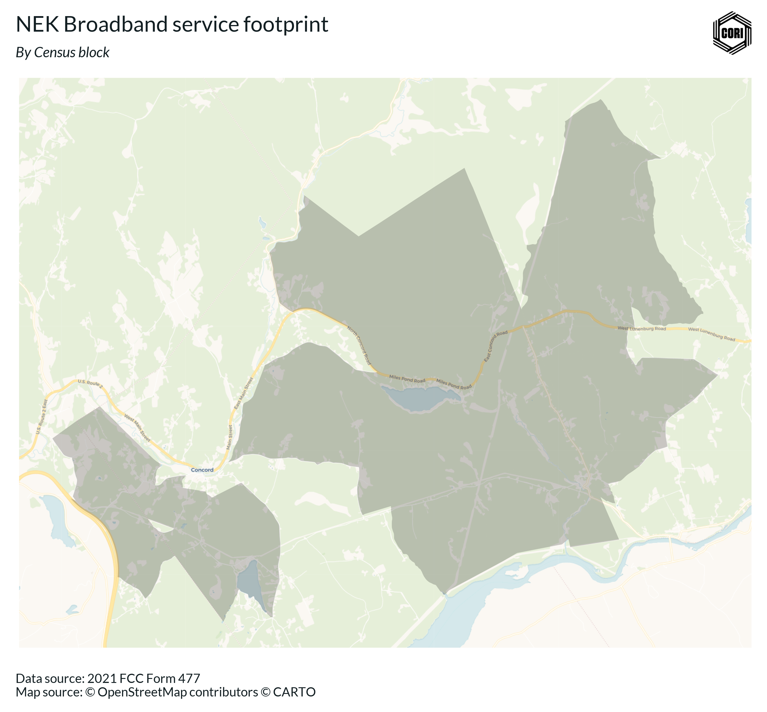
Let’s dig deeper and see what service levels NEK Broadband reports that they provide.
fig <- ggplot(data = nek_service_blocks) +
  base_map(
    st_bbox(nek_service_blocks),
    increase_zoom = 3,
    basemap = 'voyager'
  ) +
  geom_sf(aes(fill = pct_fiber), color = "black", linewidth = 0, alpha = .7) +
  scale_fill_cori(
    discrete = FALSE,
    palette = "ctg2pu",
    labels = scales::label_percent(),
    reverse = TRUE
  ) +
  theme_cori_map() +
  theme(
    legend.key.width = unit(40, "pt")
  ) +
  labs(
    title = "NEK Broadband fiber service",
    subtitle = "By Census block",
    x = NULL,
    y = NULL,
    caption = "Data source: 2021 FCC Form 477\nMap source: © OpenStreetMap contributors © CARTO",
  )

save_plot(fig, here("images/nek_broadband_fiber_service.png"), chart_height = 9)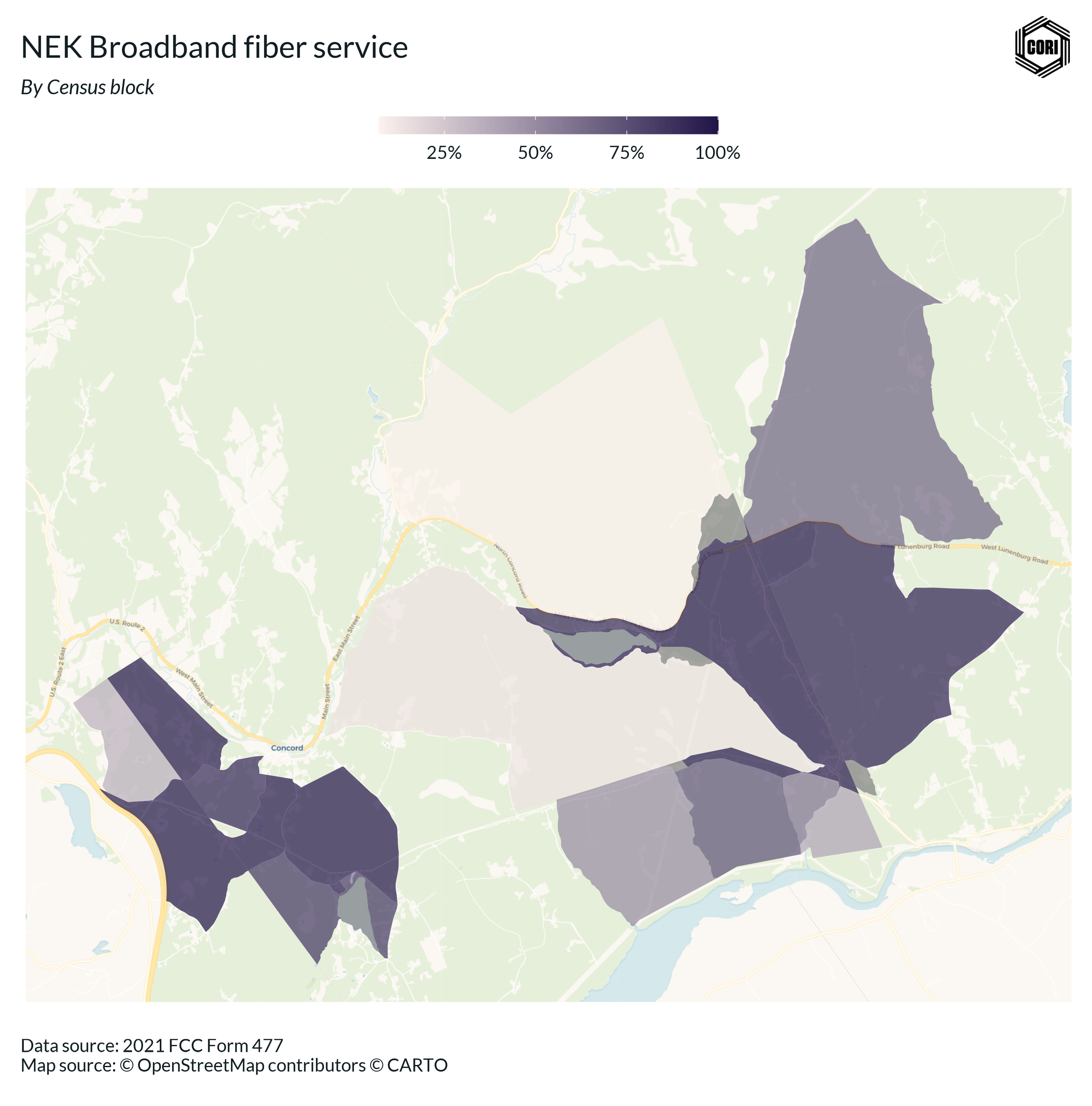
3. Compare service over time
Finally, we can use cori.data.fcc to see how reported broadband service levels vary over time.
To do so, we will use the get_county_nbm_raw function to load data for Caledonia County, VT from the 2022 and 2023 December NBM releases.
# See what NBM releases are available
available_releases <- get_nbm_release()

caledonia_2023 <- get_county_nbm_raw("50005", frn = "all", release = "2023-12-01") %>%
  mutate(year = 2023)
caledonia_2022 <- get_county_nbm_raw("50005", frn = "all", release = "2022-12-01") %>%
  mutate(year = 2022)

caledonia_combined <- bind_rows(
  caledonia_2022,
  caledonia_2023
)
The raw county data reports service levels for every broadband serviceable location. To create block totals, we will need to do some aggregation calculations.
# Calculate the percent of locations with at least 100/20 Mbps service
caledonia_chg <- caledonia_combined %>%
  mutate(
    has_100_20_service = ifelse(
      max_advertised_download_speed >= 100 &
        max_advertised_upload_speed >= 20,
      1,
      0
    )) %>%
  mutate(
    valid_100_20_location = ifelse(has_100_20_service == 1, location_id, NA)
  ) %>%
  # Filter out satellite coverage which overstates service levels
  dplyr::filter(!technology %in% c("61", "60")) %>%
  group_by(geoid_bl, year) %>%
  summarise(
    # number of locations that have 100/20 service
    count_100_20 = n_distinct(valid_100_20_location, na.rm = TRUE),
    # number of location
    count_total = n_distinct(location_id),
    # number of services
    n_services = n()
  ) %>%
  mutate(
    pct_100_20 = count_100_20 / count_total
  ) %>%
  select(geoid_bl, count_100_20, count_total, n_services, pct_100_20, year)

# Combine with tigris spatial data to get our data ready for mapping
caledonia_blocks <- tigris::blocks("50", county = "005")

chrt_dta <- left_join(
    caledonia_blocks,
    caledonia_chg,
    by = c("GEOID20" = "geoid_bl")
  ) %>%
  filter(!is.na(year))
Now our data is ready to map!
fig <- ggplot(data = chrt_dta) +
  base_map(
    st_bbox(chrt_dta),
    increase_zoom = 3,
    basemap = 'voyager'
  ) +
  geom_sf(aes(fill = pct_100_20), color = "black", linewidth = .05, alpha = .7) +
  scale_fill_cori(
    discrete = FALSE,
    palette = "ctg2pu",
    labels = scales::label_percent(),
    reverse = TRUE
  ) +
  theme_cori_map() +
  theme(
    legend.key.width = unit(40, "pt"),
    strip.text = element_text(face = "bold", size = 12)
  ) +
  labs(
    title = "Caledonia County broaband service over time",
    subtitle = "Percent of locations with 100/20 Mbps broadband service, by Census block",
    x = NULL,
    y = NULL,
    caption = "Data source: 2022 and 2023 FCC NBM\nMap source: © OpenStreetMap contributors © CARTO",
  ) +
  facet_wrap(~year, ncol = 2)

save_plot(fig, here("images/caledonia_broadband_100_20_service.png"), chart_height = 8.5)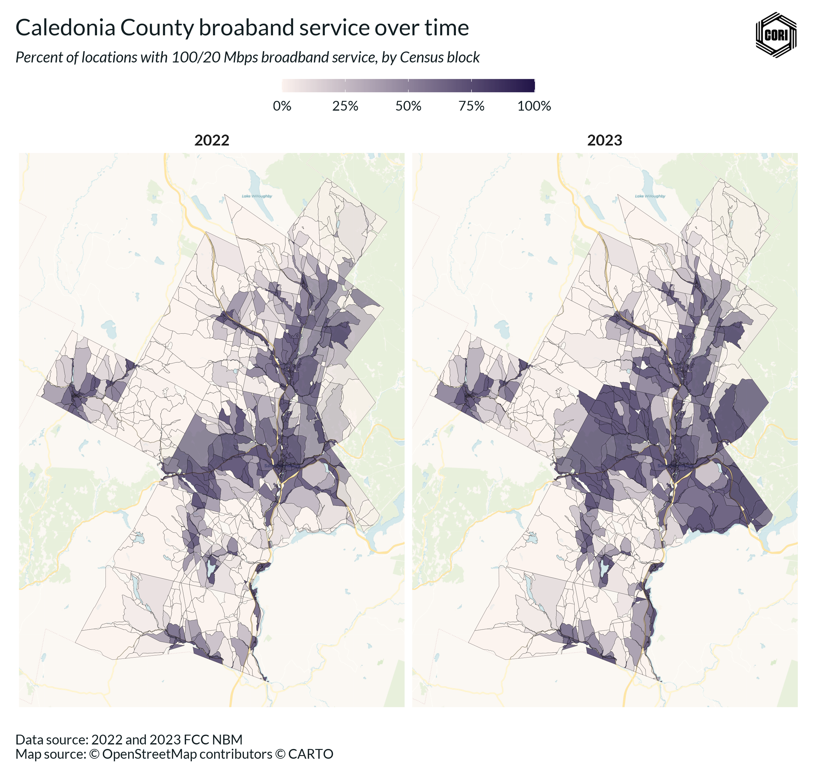
There’s a lot more to discover in the package, so I highly recommend you check out the reference documentation and give it a try yourself.